Activity 15 - Neural Networks

A neural network is typically a computational model which mimics the processing model of the neurons in the human brain. The 'neurons' on said network has an advantage over Linear Discriminant Analysis in that it does not require a given boundaries or rules in order to perform the classification, it 'learns' these rules for itself through a given set of weighed inputs.

Fig. 1. Artificial Neural Network [1]

Consider the figure above, let us consider that the input is a vector and each given input node represents one dimension of the vector. Each input is given a given weight, and when processed gives out a variable a. This variable act on the activation function g, which gives the output z. This model describes the basic mechanics of a feedforward neural network. For this activity the Artificial Neural Network toolbox for Scilab was downloaded and the feature data from Activity 14 was used. 

A feedforward neural network was created, 3 feature data was used as input, run through one hidden layer, and the resulting classification would be represented in the form of three binary digits.

0 1 0 - green rectangle

1 0 0 - red rectangle

1 1 0 - yellow rectangle

0 1 1 - green circle

1 0 1 - red circle

The same training population was used and same number of instances were used for classification. A learning rate of 2.5 with the network trained for 400 repetitions for the weight. Using this process a 100% rate of classification was achieved when performed for 50 repetitions with random training population sampling.

I would like to give myself a grade of 10 for this activity for understanding and implementing the needed procedure.

Reference:

[1] M. Soriano, 'Neural Networks', Applied Physics 186 Activity Manual 2013

Activity 14 - Pattern Recognition

Human vision allows for color constancy which allows the perception of the same color of an object even if illuminated by different sources. Though color constancy alone is not responsible for object identification, humans also rely heavily on pattern recognition, which can be as simple as that most apples are red, coins are circular and has a metallic texture, or as complex as leaf patterns, and hand writing patterns. For this to be done digitally through code, feature extraction must be performed first and then categorization.

On deciding on what image features to extract from the object, it would be more efficient to only acknowledge distinguishing features among the object which one wishes to classify. Thus for this activity I will be classifying the objects shown in Figure 1. The images are composed of generally circular and rectangular shaped cut outs of varying colors dominant along the red and green hues.

Figure 1. Cut outs taken into consideration for classification

To do this I will be extracting three features, namely RGB values, preferably for the red and green channel, and area estimation of each sample. In order to do this, each sample from the images has to be isolated, thus a good contrast between the object and the background would be a good starting point to segment the cutouts.

Figure 2. Original data subject to be categorized, but background provided poor contrast for segmentation. (Left) Shotgun Shells. (Middle and Right) Pistol bullet cartridges

After they are segmented, one performs blob analysis, using SearchBlobs() function, so as to be able to call on the blobs one-by-one for feature extraction. Thus to do this, area calculation was performed the same as that performed in Activity 5, particularly pixel counting, while green and red channel value value extraction was performed as the mean value of the corresponding color channels of the detected blobs. With texture extraction complete, we can now do pattern recognition. First, a sample set is used to train the code while the remaining samples are used to test if the classification is a success. If not, then the set of features used needs to be changed or additional features are added to have a higher success rate. Note that one should refrain from using all data set for training to avoid 'memorization' of data rather than pattern recognition. For this activity I will be using 75% of the data set as training set while the remaining 25% as the test samples.

Figure 3. 3D scatter plot of the feature values

Shown in the Figure above is the 3D scatter plot of the three features chosen, as can be seen the groups are neatly separated. Now if we are to classify the remaining data set into their corresponding groups there are many methods that can be implemented, of which include the metric distance and linear discriminant analysis (LDA). Initially I will only be performing the metric distance method but if I would include the LDA latter on. For the metric distance method, one can perform either the K-nearest neighbor (k-nn) rule using euclidean distance or the Mahalanobis distance algorithm. For simplicity, I will be using the k-nn rule; in this method the euclidean distance was calculated between the texture values of the object to be classified, known as Instance, from all the training data set. The nearest k neighbors are taken as votes, the group with the most number of votes is where the instance will be classified into. k is preferably an odd numbered integer as to avoid a tie between vote. For this activity 16 samples represent each group, with 12 used as training data set, and 4 to be classified per group; k = 11.

Applying the method mentioned above, 18 out of the 20 data samples were correctly classified, giving an accuracy of 90%. But from where could have the error arisen from? Looking back into the features taken into account, it can be seen that the distance measurement is heavily dependable on the pixel area in terms of the magnitude of values. Thus to equally distribute the weights of each feature, these values has to be normalized. Doing this corrects the error observed earlier and a perfect classification is achieved.

Figure 4. Normalized feature values

For this activity I give myself a grade of 10 for completing the activity and performing the necessary applications.

Activity 13 - Image compression

In this activity we were to use Principal Component Analysis (PCA) in image reconstruction. PCA is a mathematical procedure that utilizes the orthogonal transformation to transform a set of possibly correlated variables into a smaller set of linearly uncorrelated variables which are called principal components. The principal components are ordered such that the first PC accounts for the highest variability in the data and each succeeding component has a higher variability than the next. 

In Scilab 5.4.1, the PCA can be performed by calling the pca(x) function. The output of the function is separated into three matrixes depending upon the variable names given. Following the default given by the demo, we shall call them lambda, facpr, and comprinc.  The input x is an n x p matrix wherein there are n observations with p components. The outputs lambda is a p x 2 matrix where the first column contains the correlation, and the second column contains the percentage variability of the PC. The facpr contains the principal components, or the eigenvalues, while comprinc contains the projections of each observation towards the PC. In this activity, the components for reconstruction is encased in the facpr matrix.

In order to perform the image compression, a template has to be set such that the image can be reconstructed. Thus in this activity the image shown below was used. Both are already scaled images, the first a 500 x 375 image while the second is a 510 x 248 image. The image is then partitioned into individual 10 x 10 blocks to act as the individual observations. With the observations to be in vector form, the 10 x 10 blocks were concatenated into 1 x 100 matrices and all observations were contained in the r*c x 100 matrix x, where r and c are the dimensions of the image. The principal components were thus calculated by using the pca() function.

Using the cumsum() function upon the second column in lambda, I can tell the degree of reconstruction done by using the combined weighted eigenimages in facpr. The weight themselves are computed as the scalar dot multiplication of the concatenated 10 x 10 image block and the corresponding eigenimage. As can be seen, the method implied works best for a 2D image, as such this was tested on the grayscale image of the kite.

The eigenimages and their corresponding weights were calculated as discussed earlier. The images were reconstructed from least (72%) to greatest (100%) in iterations of 4%. The minimum reconstruction will inevitably depend the highest variability of the eigenimages. As can be seen with the images below.

For size comparison refer to the table shown below, the size of the image cropped to the same size as the reconstructed image is 92.1 kB.

As can be seen, image size decreases between 92% to 96% reconstruction, but my take on this is that at the 92% percent reconstruction, pixelation of the image decreased which could have decreased the data load in the matrix. With that an image reconstruction has been performed on a grayscale image. On a colored image though this can be done by performing the reconstruction per color channel and combining the results in order to form the RGB image.

Due to the compresion, the 96% reconstruction looks similar to the 100% reconstruction. Again as shown in the table below, the image size decreases correspondingly to the percentage of reconstruction. Size of the original image cropped to the same dimensions is 456 kB.

In this activity I give myself a grade of 11 for being able to complete the activity and for being able to to the method on a colored image.

Activity 12 - Playing notes by Image Processing

Utilizing all the skills acquired in the previous 11 activities, for this activity we were analyze a digital copy of a music sheet and play the notes accordingly using Scilab. For this activity I chose the musical sheet of Frere Jacques:

As one can see, it is a simple music sheet composed of six notes, incorporating Do to La, separated into three different durations (half, quarter, and half-quarter).  The first step would be apply a threshold unto the image.

From here I have to determine the location of the notes and the pixel coordinates denoted by the bar to identify the half-quarter notes, I will refer to the notes by their time duration. I decide to tackle the detection of the notes first. Since the notes are nearly circular, they can be isolated by performing a Open morphological operation with a circle of a radius of 1.

Figure 1. Image after morphological operation 

FilterBySize() was then applied to remove the small dots and other unnecessary objects, and since the limit of the ledge lines are known, I can impose a zero value to those above it.

As can be seen the notes has been isolated. I then have to separate the half-note from the others. A key factor in doing this is blob size, as the half notes should have a lesser blob size. Using SearchBlob() as to identify each individual blob and determining their size, I then utilize the histplot() function,

Figure 2. Pixel area distribution

Thus pixel areas less than 100 belong to the half-note, while those above it are to be considered to be of the quarter notes and half-quarter note. Thus by again utilizing the FilterBySize() function, I can separate the two.

For the half note, an Closing morphological operation has to be applied to close the gap between the notes, after doing so the center coordinates for both note categories could be detected by taking the average coordinates of each blob.

Figure 3. Plot of note coordinates

With the notes categorized according to height and location, they can now be classified according to their pitch. For this I use the Key of C of the 3rd octave. The only problem now is classifying them according to their duration, with the half notes identified, I now only have to differentiate between the quarter note and half-quarter note. Referring to Figure 1, the half-quarter note is denoted by a bar, thus by determining the column coordinates of the bar and adjusting it accordingly in reference to the last note, notes detected lying along these coordinates are identified as half-quarter notes.

There are two ways in order to do this, one is by applying FilterBySize() once again to isolate the bar,

Or one can apply correlation via Fourier Transform with the bar as the patter,

Thus by reconstructing the notes in audio as sine waves:

        note = sine(2*f*t*pi)

I was able to play the music sheet via Scilab. I saved the music file as a video using Windows Live movie Maker following this steps.

I have uploaded the video in youtube.

For this I would like to give myself a grade of 11, for being able to apply the code correspondingly and doing what was required. The additional point was for being able to create a video of the audio file. :)

References:
[1] M. Soriano, 'Activity 12 - Playing notes by Image Processing', Applied Physics 186 manual. UP Diliman, Quezon.
[2]http://www.vaughns-1-pagers.com/music/musical-note-frequencies.htm. Retrieved on August 28, 2013
[3]https://support.google.com/youtube/answer/1696878?topic=2888648&hl=en-GB. Retrieved on August 29, 2013

Activity 11 - Application of Binary Operations 1

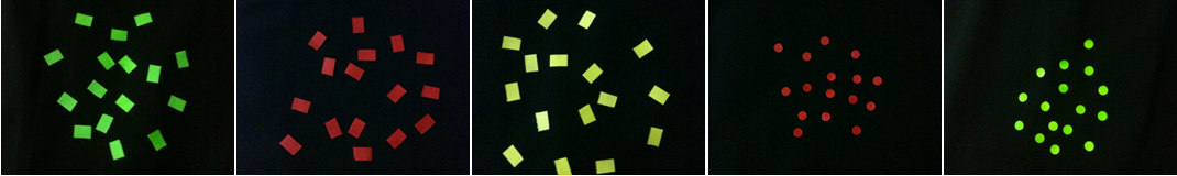
In this activity, we were task in implementing past activity knowledge into object detection.segmentation. We were given two images shown in Figure 1 and 2.

Figure 1. Normal sized cells

Figure 2. Normal sized cells with five Abnormal Sized cells marked red

In figure 1, we are to assume each punched paper as normal cells. As can be seen, some of the cells overlap in pairs and in groups. For the first image, the goal would be to determine the best estimate of pixel area of one cell represented in terms of mean and standard deviation. Using these values, the abnormal sized cells in Figure 2 are to be isolated.

Thus the first step to be taken was to perform a threshold on the image. Analyzing the histogram of the image, thresholds were tested for values ranging from 170-210 and it was determined that 200 would be the best choice based on the result. As can be seen, the thresholded image has kept most of the cells circular in shape though a large part of the background was also detected in the right side of the picture, this will be removed later on after Morphological Operations.

Figure 3. Histogram of Figure 2.

Figure 4. After application of threshold

Given that the object of interest is circular, then the ideal Structuring Element should also be circular. Open function should therefor be implemented to filter out the background pixels via erosion while reconstructing the circular blobs through Dilation. Performing this, most of the imperfect cells, background image, as well as most of the cell outline are removed. In this activity, a circle structure element of size 12 was implemented.

Figure 5. (Left) Image after applying OpenImage. (Middle) Filtered out part of Figure 4. (Right) Detected cells in original image

FilterBySize() function was then used as a precautionary measure to remove any unwanted background pixel that wasn't filtered out; minimum pixel size was set to 100. Note that before this was applied, SearchBlobs() function was applied first. Thus each individual blob is marked by a separate value, summing the number of pixels corresponding to each blob value will give the pixel area of each blob. Doing this for the result in Figure 5, I was able to determine the pixel area of all 49 detected blobs in the image. Based from Figure 5, it can be seen that there are 10 blobs with overlapping cells, thus this cells should have a noticeable enlargement in pixel area compared to the other blobs corresponding to singular cells. This is shown in Figure 7, comparing the histogram with the image shown it can be assumed that blobs with pixel size greater than 600 do not belong to the singular cell group. Applying this via FilterBySize() function proves accurate. Thus calculating the mean and standard deviation of the pixel size shows that mean, µ = 498.35 pixels and standard deviation, σ = 24.28 pixels. Based from this the range of values corresponding to a normal sized cell is (µ +/- 3*σ) pixels or 425 - 571 pixels. Based from this overlapping pairs of pixels can be assumed to be twice the pixel area of an individual normal sized cell, 600 - 1000 pixels. While overlapping cells in groups of three or more should be greater than 1000. Which can be seen to apply for the detected blobs as shown in Figure 9.

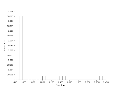
Figure 6. Histogram of Pixel Area of all detected blobs

Figure 7. Marked overlapping cells

Figure 8. (Left) Histogram of values corresponding to individual normal cells. (Right) Detected individual normal cells

Figure 9. After applying FilterBySize(Image, min, max). (Left) min = 600, max = 1000. (Right) min = 1000, max = infinity

Applying the same procedure for the image in Figure 2, filtering out the individual cells via FilterBySize() function by setting the minimum size as 571, I was able to get the abnormal sized cells along with overlapping cells. By filtering out overlapping cells in groups of three or more, only the abnormal size cells and the overlapping cell pair remains. Analyzing the histogram, it was observed that the pixel area of the abnormal sized cells corresponds with overlapping cell pairs. Thus the only other way of removing the overlapping pair from the image, aside from recreating a more complex morphological operation, was to implement a larger circular structure element such that normal sized cell would not be able to fit but abnormal sized cells would. Thus a circular structure element of size 13 was implemented.

Figure 10. After applying FilterBySize(Image, min, max). (Left) min = 571 (Right) min = 571, max = 1000

Figure 11. (Left) After applying new Structure element (Right) Inverting detected blobs and superimposing on original image

As can be seen the abnormal sized cells were isolated. In this activity, it was advised that the image in Figure 1 be divided into subimages and average the pixel area of the detected blobs to act as the average normal size of an individual cell. But this was determined via a different method in this activity. Nonetheless, I would like to give myself a grade of 10 for being able to complete the Activity and being able to understand what has been done. I am aware that I could done a better job at separating the blobs if a more thorough implementation of morphological operation was applied.

References:

M. Soriano, "Activity 11 - Application of Binary Operations 1". Applied Physics 186 2013. NIP, University of the Philippines -Diliman.

Activity 10 - Morphological Operation

Morphology refers to shape or structure. In image processing, morphological operations are usually performed on binary images, where the data formation of 1's are of interest, so as to improve the image or to extract information, i.e. Isolation and Detection of Spectral line. Thus by this notion, morphological operation affects the shape of the image. In implementing Morphological operations, it is essential to understand set theory.

If assume A to be a set in 2D interger space, and let a be an element of A, then this is represented as,

and if we assume an element b  set B which is not found in set A then

 If however we want to denote A as a subset of B then

which denotes that all elements of A can be found in B but not otherwise. 

Set operations on the other hand include union, which is a set containing all elements contained in the two sets related to the operation, denoted by:

while an intersection denotes a set that contains identical elements between two sets denoted by:

If, however, the two sets are mutually exclusive or that they have no common elements, then the resulting intersection between the two would be result in a null set, shown as:

A complement of A is a set which contains all elements not present in A is denoted as:

the last two set operation are reflection, or flipping the set, and translation, denoted as:

respectively.

In morphological operation, two basic techniques are the dilation and erosion. Dilation is denoted as:

which denotes that the operation is a dilation of A by B. Mathematically, the operation is read such that the structuring element, B, is reflected and will involve all z's such that the intersection of A and the translation of the reflected B does not result in a null set. Thus the effect of Dilation either expands or elongates the image. Erosion on the other hand is denoted by:

which reads as the erosion of A by B. The operation involves all z's such that B translated by z is contained in A or will result such that B will become a subset of A.

Dilation and Erosion can thus be performed manually. In this activity Dilation and Erosion were performed on the following images:

Figure 1. (Leftmost) 5x5 Square (Middle Left) Right Triangle with base = 4 and height = 3 (Middle Right) 10x10 Hollow square with a thickness of 2 pixels and (Rightmost) Plus sign 5 pixels across with 1 pixel thickness

 Using the following structuring elements:

Figure 2. (Leftmost) 2x2 Square (Middle Left) 2x1, (Middle) 1x2 (Middle Right) Plus sign 3 pixels across (Rightmost) 2x2 Diagonal

Implementing each and every Structure element per image, manually through Excel and automatically through Scilab, we compare the results.

 

Figure 3. Solid Square (Top) Manual Dilation and Erosion. (Bottom) Through Scilab

Figure 4. Triangle (Top) Manual Dilation and Erosion. (Bottom) Through Scilab

Figure 5. Hollow Square (Top) Manual Dilation and Erosion. (Bottom) Through Scilab

Figure 5. Plus (Top) Manual Dilation and Erosion. (Bottom) Through Scilab

As can be seen, the results are exact for the application of Erosion and differ for the Dilation. In my perspective, it seems that the dilation of Scilab did not apply reflection during dilation and as such the difference observed above. 

I would like to apologize for the late submission which was caused by faulty internet connection.

Reference:

[1] M. Soriano. "Morphological Operations". Applied Physics 186 2013. University of the Philippines