Activity 12 - Playing notes by Image Processing

Utilizing all the skills acquired in the previous 11 activities, for this activity we were analyze a digital copy of a music sheet and play the notes accordingly using Scilab. For this activity I chose the musical sheet of Frere Jacques:

As one can see, it is a simple music sheet composed of six notes, incorporating Do to La, separated into three different durations (half, quarter, and half-quarter).  The first step would be apply a threshold unto the image.

From here I have to determine the location of the notes and the pixel coordinates denoted by the bar to identify the half-quarter notes, I will refer to the notes by their time duration. I decide to tackle the detection of the notes first. Since the notes are nearly circular, they can be isolated by performing a Open morphological operation with a circle of a radius of 1.

Figure 1. Image after morphological operation 

FilterBySize() was then applied to remove the small dots and other unnecessary objects, and since the limit of the ledge lines are known, I can impose a zero value to those above it.

As can be seen the notes has been isolated. I then have to separate the half-note from the others. A key factor in doing this is blob size, as the half notes should have a lesser blob size. Using SearchBlob() as to identify each individual blob and determining their size, I then utilize the histplot() function,

Figure 2. Pixel area distribution

Thus pixel areas less than 100 belong to the half-note, while those above it are to be considered to be of the quarter notes and half-quarter note. Thus by again utilizing the FilterBySize() function, I can separate the two.

For the half note, an Closing morphological operation has to be applied to close the gap between the notes, after doing so the center coordinates for both note categories could be detected by taking the average coordinates of each blob.

Figure 3. Plot of note coordinates

With the notes categorized according to height and location, they can now be classified according to their pitch. For this I use the Key of C of the 3rd octave. The only problem now is classifying them according to their duration, with the half notes identified, I now only have to differentiate between the quarter note and half-quarter note. Referring to Figure 1, the half-quarter note is denoted by a bar, thus by determining the column coordinates of the bar and adjusting it accordingly in reference to the last note, notes detected lying along these coordinates are identified as half-quarter notes.

There are two ways in order to do this, one is by applying FilterBySize() once again to isolate the bar,

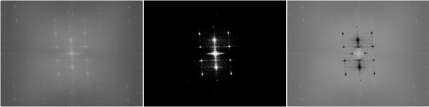
Or one can apply correlation via Fourier Transform with the bar as the patter,

Thus by reconstructing the notes in audio as sine waves:

        note = sine(2*f*t*pi)

I was able to play the music sheet via Scilab. I saved the music file as a video using Windows Live movie Maker following this steps.

I have uploaded the video in youtube.

For this I would like to give myself a grade of 11, for being able to apply the code correspondingly and doing what was required. The additional point was for being able to create a video of the audio file. :)

References:
[1] M. Soriano, 'Activity 12 - Playing notes by Image Processing', Applied Physics 186 manual. UP Diliman, Quezon.
[2]http://www.vaughns-1-pagers.com/music/musical-note-frequencies.htm. Retrieved on August 28, 2013
[3]https://support.google.com/youtube/answer/1696878?topic=2888648&hl=en-GB. Retrieved on August 29, 2013

Activity 11 - Application of Binary Operations 1

In this activity, we were task in implementing past activity knowledge into object detection.segmentation. We were given two images shown in Figure 1 and 2.

Figure 1. Normal sized cells

Figure 2. Normal sized cells with five Abnormal Sized cells marked red

In figure 1, we are to assume each punched paper as normal cells. As can be seen, some of the cells overlap in pairs and in groups. For the first image, the goal would be to determine the best estimate of pixel area of one cell represented in terms of mean and standard deviation. Using these values, the abnormal sized cells in Figure 2 are to be isolated.

Thus the first step to be taken was to perform a threshold on the image. Analyzing the histogram of the image, thresholds were tested for values ranging from 170-210 and it was determined that 200 would be the best choice based on the result. As can be seen, the thresholded image has kept most of the cells circular in shape though a large part of the background was also detected in the right side of the picture, this will be removed later on after Morphological Operations.

Figure 3. Histogram of Figure 2.

Figure 4. After application of threshold

Given that the object of interest is circular, then the ideal Structuring Element should also be circular. Open function should therefor be implemented to filter out the background pixels via erosion while reconstructing the circular blobs through Dilation. Performing this, most of the imperfect cells, background image, as well as most of the cell outline are removed. In this activity, a circle structure element of size 12 was implemented.

Figure 5. (Left) Image after applying OpenImage. (Middle) Filtered out part of Figure 4. (Right) Detected cells in original image

FilterBySize() function was then used as a precautionary measure to remove any unwanted background pixel that wasn't filtered out; minimum pixel size was set to 100. Note that before this was applied, SearchBlobs() function was applied first. Thus each individual blob is marked by a separate value, summing the number of pixels corresponding to each blob value will give the pixel area of each blob. Doing this for the result in Figure 5, I was able to determine the pixel area of all 49 detected blobs in the image. Based from Figure 5, it can be seen that there are 10 blobs with overlapping cells, thus this cells should have a noticeable enlargement in pixel area compared to the other blobs corresponding to singular cells. This is shown in Figure 7, comparing the histogram with the image shown it can be assumed that blobs with pixel size greater than 600 do not belong to the singular cell group. Applying this via FilterBySize() function proves accurate. Thus calculating the mean and standard deviation of the pixel size shows that mean, µ = 498.35 pixels and standard deviation, σ = 24.28 pixels. Based from this the range of values corresponding to a normal sized cell is (µ +/- 3*σ) pixels or 425 - 571 pixels. Based from this overlapping pairs of pixels can be assumed to be twice the pixel area of an individual normal sized cell, 600 - 1000 pixels. While overlapping cells in groups of three or more should be greater than 1000. Which can be seen to apply for the detected blobs as shown in Figure 9.

Figure 6. Histogram of Pixel Area of all detected blobs

Figure 7. Marked overlapping cells

Figure 8. (Left) Histogram of values corresponding to individual normal cells. (Right) Detected individual normal cells

Figure 9. After applying FilterBySize(Image, min, max). (Left) min = 600, max = 1000. (Right) min = 1000, max = infinity

Applying the same procedure for the image in Figure 2, filtering out the individual cells via FilterBySize() function by setting the minimum size as 571, I was able to get the abnormal sized cells along with overlapping cells. By filtering out overlapping cells in groups of three or more, only the abnormal size cells and the overlapping cell pair remains. Analyzing the histogram, it was observed that the pixel area of the abnormal sized cells corresponds with overlapping cell pairs. Thus the only other way of removing the overlapping pair from the image, aside from recreating a more complex morphological operation, was to implement a larger circular structure element such that normal sized cell would not be able to fit but abnormal sized cells would. Thus a circular structure element of size 13 was implemented.

Figure 10. After applying FilterBySize(Image, min, max). (Left) min = 571 (Right) min = 571, max = 1000

Figure 11. (Left) After applying new Structure element (Right) Inverting detected blobs and superimposing on original image

As can be seen the abnormal sized cells were isolated. In this activity, it was advised that the image in Figure 1 be divided into subimages and average the pixel area of the detected blobs to act as the average normal size of an individual cell. But this was determined via a different method in this activity. Nonetheless, I would like to give myself a grade of 10 for being able to complete the Activity and being able to understand what has been done. I am aware that I could done a better job at separating the blobs if a more thorough implementation of morphological operation was applied.

References:

M. Soriano, "Activity 11 - Application of Binary Operations 1". Applied Physics 186 2013. NIP, University of the Philippines -Diliman.

Activity 10 - Morphological Operation

Morphology refers to shape or structure. In image processing, morphological operations are usually performed on binary images, where the data formation of 1's are of interest, so as to improve the image or to extract information, i.e. Isolation and Detection of Spectral line. Thus by this notion, morphological operation affects the shape of the image. In implementing Morphological operations, it is essential to understand set theory.

If assume A to be a set in 2D interger space, and let a be an element of A, then this is represented as,

and if we assume an element b  set B which is not found in set A then

 If however we want to denote A as a subset of B then

which denotes that all elements of A can be found in B but not otherwise. 

Set operations on the other hand include union, which is a set containing all elements contained in the two sets related to the operation, denoted by:

while an intersection denotes a set that contains identical elements between two sets denoted by:

If, however, the two sets are mutually exclusive or that they have no common elements, then the resulting intersection between the two would be result in a null set, shown as:

A complement of A is a set which contains all elements not present in A is denoted as:

the last two set operation are reflection, or flipping the set, and translation, denoted as:

respectively.

In morphological operation, two basic techniques are the dilation and erosion. Dilation is denoted as:

which denotes that the operation is a dilation of A by B. Mathematically, the operation is read such that the structuring element, B, is reflected and will involve all z's such that the intersection of A and the translation of the reflected B does not result in a null set. Thus the effect of Dilation either expands or elongates the image. Erosion on the other hand is denoted by:

which reads as the erosion of A by B. The operation involves all z's such that B translated by z is contained in A or will result such that B will become a subset of A.

Dilation and Erosion can thus be performed manually. In this activity Dilation and Erosion were performed on the following images:

Figure 1. (Leftmost) 5x5 Square (Middle Left) Right Triangle with base = 4 and height = 3 (Middle Right) 10x10 Hollow square with a thickness of 2 pixels and (Rightmost) Plus sign 5 pixels across with 1 pixel thickness

 Using the following structuring elements:

Figure 2. (Leftmost) 2x2 Square (Middle Left) 2x1, (Middle) 1x2 (Middle Right) Plus sign 3 pixels across (Rightmost) 2x2 Diagonal

Implementing each and every Structure element per image, manually through Excel and automatically through Scilab, we compare the results.

 

Figure 3. Solid Square (Top) Manual Dilation and Erosion. (Bottom) Through Scilab

Figure 4. Triangle (Top) Manual Dilation and Erosion. (Bottom) Through Scilab

Figure 5. Hollow Square (Top) Manual Dilation and Erosion. (Bottom) Through Scilab

Figure 5. Plus (Top) Manual Dilation and Erosion. (Bottom) Through Scilab

As can be seen, the results are exact for the application of Erosion and differ for the Dilation. In my perspective, it seems that the dilation of Scilab did not apply reflection during dilation and as such the difference observed above. 

I would like to apologize for the late submission which was caused by faulty internet connection.

Reference:

[1] M. Soriano. "Morphological Operations". Applied Physics 186 2013. University of the Philippines

Activity 8 - Enhancement in the Frequency Domain

This activity is focused on noise cancellation or removal in images. Main concepts to be used in this activity focuses on application of Fourier Transform via FFT in 2D space and convolution, both of which was discussed in Activity 7. But before we go into noise cancellation, we will first look into various insights into convolution and FFT.

First we synthesize a 200x200 binary image of various shapes, as shown in the top row of Figure 1. Now the first image from the left, shows two equally spaced dots, but mathematically this can be viewed as two Dirac deltas, and as such we can see that the Fourier of such an image results in a sinusoid. Though its sinusoidal pattern is not as clear as plotting it in 3D, the varying intensity of the plot should suffice in supporting the statement. Increasing the distance between the two dots would result in a higher frequency sinusoid, as would decreasing the pixel distance result in a lower frequency sinusoid. From the previous Activity it was shown that by applying fft2() to an image would give of its representation in frequency space but applying it again would revert it back to the original image. Also recall that FT represents data into its frequency components, now assuming that the two equally spaced dots represent the frequency of a sinusoidal function then applying fft2() would result in an image representing such a function, as was shown. 

Figure 1.(Top row) Synthesized images of equally spaced dots, circles, squares and Gaussians. (Bottom Row) Resulting Fourier Transform  

The second image is that of two equally spaced circles, which is a convolution of the previous spaced dirac delta and a circle. As such the resulting transform of the two should be a element-per-element multiplication of the transforms of the two images as shown in Figure 1. The output is that of a sombrero function superimposed upon a sinusoidal function which are the transform of a circle and of two Dirac deltas, respectively. This concept can also be observed in the other two images in Figure 1. The third and fourth top row image shows the convolution of a square and of a Gaussian to two Dirac deltas, respectively. Since the transform of a square is a sinc function and the transform of a Gaussian is a Gaussian the output is as shown in Figure 1. Note however that increasing the variance of the Gaussian in the input will lead to a smaller Gaussian in the frequency space and decreasing variance will result in the opposite.

The process in which the previous images can be explained by performing the following. Synthesizing 10 Diracs randomly distributed along a 200x200 black image, and a random pattern, as shown in Figure 2. Taking the transforms of the two images and performing element-by-element multiplication of the results then applying fft2() to the product would result to the image shown in Figure 3. As can be seen the pattern is superimposed on each dot from the earlier image. In the same manner, one can replicate the images in Figure 1.

Figure 2.(Left) Randomly placed Dirac Deltas. (Right) Diamond Pattern

Figure 3. Resulting Fourier Convolution of the images in Figure 2. Image was flipped for comparison.

Now implementing fft2() to equally spaced vertical lines, shown in Figure 4, will result to fringes, also shown in Figure 4. The Fourier transform sees that image as an array of equally spaced Dirac Deltas or Dirac Delta train, applying fft2() to such an array would result in a Dirac Delta train with a spacing, 1/T, equal to the inverse of the spacing in the spatial domain, T. Thus as shown in Figure 4, as the spacing between the dirac train increases, the spacing between the fringes lessens.

Figure 4. (Top Row) Equally spaced dirac trains. (Bottom Row) Fringe Patterns.

Returning to noise cancelling, noise can be defined as unwanted signal that is considered to be spurious and extraneous information, and is usually a by-product of how the image was captured. In Figure 5 for example, the image exhibits equally spaced vertical lines similar to those of Figure 4. These are the result of digitally stitching of 'framelets' in order to form the image. Analyzing the transform of the image, the fringe pattern which was shown earlier, can also be observed both horizontally and vertically. A mask or a filter was thus synthesized in order to remove the noise, which consisted of pattern much like a crosshair since the middle part of the transform has to be kept the same since low frequency is usually the domain of important image data. After performing element-per-element multiplication between the mask and the FT of the image, performing fft2() to the result gives of a filtered image without the prevalent noise observed in Figure 5.

Figure 5. Moon image with equally spaced vertical lines [2]

Figure 6. (Left) Fourier Transform of Figure 5. (Middle) Mask. (Right) Superimposed masked on FT of the Moon image

Figure 7. Filtered image after applying mask

Another way of performing this is by measuring the pixel distance between each vertical line, then from that replicate the pattern of the vertical lines. Take the transform of the pattern perform element-per-element division from the transform of the image in Figure 5, the resulting image should give an output similar or identical to that of Figure 7.

The last image to be to be subjected to noise cancellation is, shown in Figure 8, a painting by Dr. Vincent Daria. Shown in Figure 9 is the transform of the image. Since no pattern can be generated quickly, a quick way to create a mask is to threshold the transform and convert it to binary. Now getting the negative of the binary and superimposing a circle to the center and the mask for the image is complete. The result is shown in Figure 10.

Figure 8. Oil Painting by Dr. Vincent Daria

Figure 9. (Left) FT of Figure 8. (Middle) FT after applying the threshold. (Right) Filtered FT

Figure 10. Filtered image from Figure 8

In this activity I give myself a grade of 10, for completing the task and for being able to comprehend and explain the performed tasks.

Reference:
[1] M. Soriano. "Enhancement in the Frequency Domain". Applied Physics 186 2013. University of the Philippines.

[2] lpi.usra.edu. "Apollo 11 Mission". Accessed on July 30, 2013.  http://www.lpi.usra.edu/publications/slidesets/apollolanding/ApolloLanding/slide_05.html

[3] http://en.wikipedia.org/wiki/Image_noise