Images taken from environments too dim or too bright has a histogram which is more likely to be one sided. That is why in this activity we were tasked with enhancing an image via Histogram manipulation. Thus in this activity we will be applying a histogram manipulation technique known as backprojection.
The histogram of the image in grayscale is taken and normalized with the number of pixels present within the image. This normalized histogram is known as the probability distribution function (PDF). Taking the cumulative sum of the histogram, we have the cumulative distribution function (CDF) of the image. We then project the CDF of the image to a desired CDF.
Doing this in Scilab, the image of interest, shown in Figure 1, is converted into grayscale using the rgb2gray() function. At first glance, one can see that there are two people having a discussion within the image with a third sitting between them. Though due to the bright background, the camera was not able to exhibit details pertaining to the subjects except their silhouette.
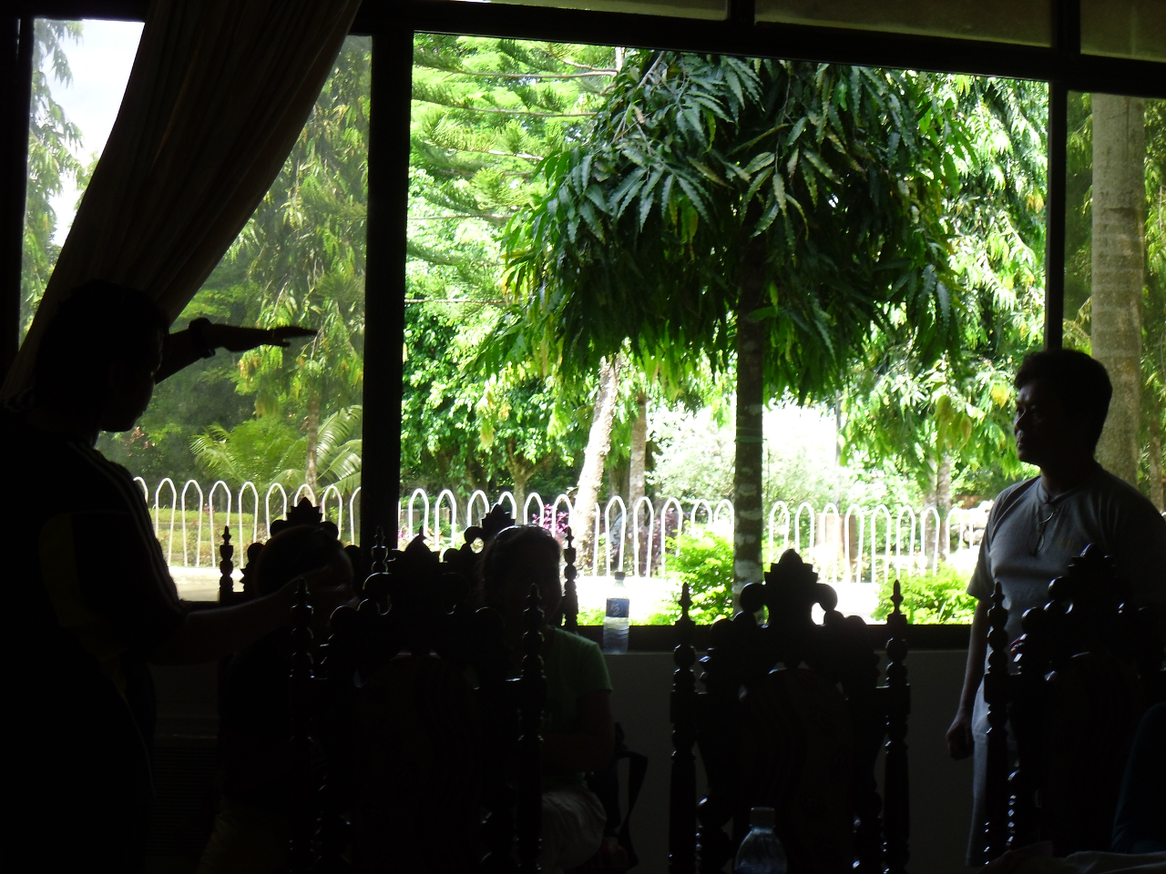
Figure 1. Image taken during a fieldwork in Samal
Details:
Dimension - 1280x960
Resolution - 96 dpi
Bit Depth - 24

Figure 2. Grayscale image of the image
The histogram of the grayscale is taken using imhist(), and normalized based from the minimum and maximum grayscale values to get the PDF.
[count, null] = imhist(gscale, 255);
counts = (counts - min(counts)/max(counts);

where in count is the array containing the histogram and eventually becomes the PDF of the image, gscale is the name of the grayscale of the image and 255 is the number of bins I want for the histogram. In this condition, pixel distribution per grayscale value is accounted for. As one can observe, the image shown is very dim due since the objects of interest were against the light. This is reflected in the histogram of the image as shown in Figure 3. From Activity 4 there were five proposed areas in the histogram; very dark, dark, neutral, bright, and very bright. From the histogram, it can be seen that the pixels are tightly spread in the very dark category of the histogram. Taking the CDF of the image by applying the cumsum() function to counts and normalizing the values results to the plot seen in Figure 4..
[count, null] = imhist(gscale, 255);
counts = (counts - min(counts)/max(counts);

Figure 3. Normalized histogram of the Image
where in count is the array containing the histogram and eventually becomes the PDF of the image, gscale is the name of the grayscale of the image and 255 is the number of bins I want for the histogram. In this condition, pixel distribution per grayscale value is accounted for. As one can observe, the image shown is very dim due since the objects of interest were against the light. This is reflected in the histogram of the image as shown in Figure 3. From Activity 4 there were five proposed areas in the histogram; very dark, dark, neutral, bright, and very bright. From the histogram, it can be seen that the pixels are tightly spread in the very dark category of the histogram. Taking the CDF of the image by applying the cumsum() function to counts and normalizing the values results to the plot seen in Figure 4..


Figure 4. CDF of the Image
What we want is an images with its pixel distribution centered about the neutral region of the histogram. This will bring out the details left out by the camera in order to adjust to the abundance of light. Thus a normalized 2D-Gaussian function was used as the ideal PDF for the image.

where sigma is the standard deviation, and a is the mean. For this image, I used a = 128 and sigma = 30. Normalizing the Gaussian function, I now have constructed the ideal PDF of my image, shown in Figure 5, followed by the ideal CDF.

Figure 5. Ideal PDF, sigma = 30 and centered at 128
Performing backtracing, I simply called out each corresponding CDF value per gray level from the image and compared it with the gray level from the ideal with the same CDF value. I replaced the image gray level with that of the ideal and processed the image.
for i = 1:length(gvalue)
[j] = find(CDFideal <= csum(i));
imp_im(find(gscale == gvalue(i))) = gvalue(j($))
end
where, imp_im is a copy of the gscale matrix I mention earlier and gvalue is the range of gray level values. At first I was implementing imp_im as a 2D matrix of zeros, but for some apparent reason the code won't work properly with this. I even tried creating imp_im as a 3D matrix of zeros and then converting it to grayscale using rgb2gray but the code still won't work. It was only when I implemented imp_im as a copy of gscale that I was finally able to produce the processed image shown in Figure 7.

Figure 6. Ideal CDF (Left) and Enhanced Image CDF (Right).

Figure 7. Original Image(Left) and Enhanced Image(Right).
Thus by using backtracking, image details that were not present in the original was shown. As one can see in the image on the right, clothing details, details on the chair, and even a fourth person was detected. This means that the camera was able to detect and retain real world object detail but was not able to exhibit it. It is to note however that there are also some features was changed in the image as emphasized by the tree in the upper left corner.
There are also other software programs which can produce the same effect as that of image backtracing. Gimp, for example, has a tool which allows manipulation of the I/O curve of the image. One simply has to load the image and convert it to grayscale as described in Activity 4. Then go to the colors menu and select curves, this will open a window showing the I/O curve of the image, which is by default, linear. Manipulating the curve, the same effects shown in Figure 7 is reproduced. Further thinkering with the I/O curve shows that its parameters are similar to that of the histogram. Increasing the values along the end of the curve increases the intensity of dark pixels while values I/O values along the end of the curve affect the intensity of the bright pixels. On a side note this can also be done for colored images, which I think is more convenient since it also adds other features into the image.

Figure 8. I/O Curve manipulation of the Image

Figure 9. I/O Curve manipulation concentrated for dark pixels of the Image

Figure 10. I/O Curve manipulation concentrated for bright pixels of the Image
Figure 11. I/O Curve manipulation concentrated for dark pixels of the Image in color
In this activity I will give myself a grade of 11, because I believe I deserve it.