Human vision allows for color constancy which allows the perception of the same color of an object even if illuminated by different sources. Though color constancy alone is not responsible for object identification, humans also rely heavily on pattern recognition, which can be as simple as that most apples are red, coins are circular and has a metallic texture, or as complex as leaf patterns, and hand writing patterns. For this to be done digitally through code, feature extraction must be performed first and then categorization.
On deciding on what image features to extract from the object, it would be more efficient to only acknowledge distinguishing features among the object which one wishes to classify. Thus for this activity I will be classifying the objects shown in Figure 1. The images are composed of generally circular and rectangular shaped cut outs of varying colors dominant along the red and green hues.
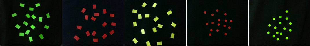
Figure 1. Cut outs taken into consideration for classification
To do this I will be extracting three features, namely RGB values, preferably for the red and green channel, and area estimation of each sample. In order to do this, each sample from the images has to be isolated, thus a good contrast between the object and the background would be a good starting point to segment the cutouts.

After they are segmented, one performs blob analysis, using SearchBlobs() function, so as to be able to call on the blobs one-by-one for feature extraction. Thus to do this, area calculation was performed the same as that performed in Activity 5, particularly pixel counting, while green and red channel value value extraction was performed as the mean value of the corresponding color channels of the detected blobs. With texture extraction complete, we can now do pattern recognition. First, a sample set is used to train the code while the remaining samples are used to test if the classification is a success. If not, then the set of features used needs to be changed or additional features are added to have a higher success rate. Note that one should refrain from using all data set for training to avoid 'memorization' of data rather than pattern recognition. For this activity I will be using 75% of the data set as training set while the remaining 25% as the test samples.

Shown in the Figure above is the 3D scatter plot of the three features chosen, as can be seen the groups are neatly separated. Now if we are to classify the remaining data set into their corresponding groups there are many methods that can be implemented, of which include the metric distance and linear discriminant analysis (LDA). Initially I will only be performing the metric distance method but if I would include the LDA latter on. For the metric distance method, one can perform either the K-nearest neighbor (k-nn) rule using euclidean distance or the Mahalanobis distance algorithm. For simplicity, I will be using the k-nn rule; in this method the euclidean distance was calculated between the texture values of the object to be classified, known as Instance, from all the training data set. The nearest k neighbors are taken as votes, the group with the most number of votes is where the instance will be classified into. k is preferably an odd numbered integer as to avoid a tie between vote. For this activity 16 samples represent each group, with 12 used as training data set, and 4 to be classified per group; k = 11.
Applying the method mentioned above, 18 out of the 20 data samples were correctly classified, giving an accuracy of 90%. But from where could have the error arisen from? Looking back into the features taken into account, it can be seen that the distance measurement is heavily dependable on the pixel area in terms of the magnitude of values. Thus to equally distribute the weights of each feature, these values has to be normalized. Doing this corrects the error observed earlier and a perfect classification is achieved.


Figure 2. Original data subject to be categorized, but background provided poor contrast for segmentation. (Left) Shotgun Shells. (Middle and Right) Pistol bullet cartridges
After they are segmented, one performs blob analysis, using SearchBlobs() function, so as to be able to call on the blobs one-by-one for feature extraction. Thus to do this, area calculation was performed the same as that performed in Activity 5, particularly pixel counting, while green and red channel value value extraction was performed as the mean value of the corresponding color channels of the detected blobs. With texture extraction complete, we can now do pattern recognition. First, a sample set is used to train the code while the remaining samples are used to test if the classification is a success. If not, then the set of features used needs to be changed or additional features are added to have a higher success rate. Note that one should refrain from using all data set for training to avoid 'memorization' of data rather than pattern recognition. For this activity I will be using 75% of the data set as training set while the remaining 25% as the test samples.
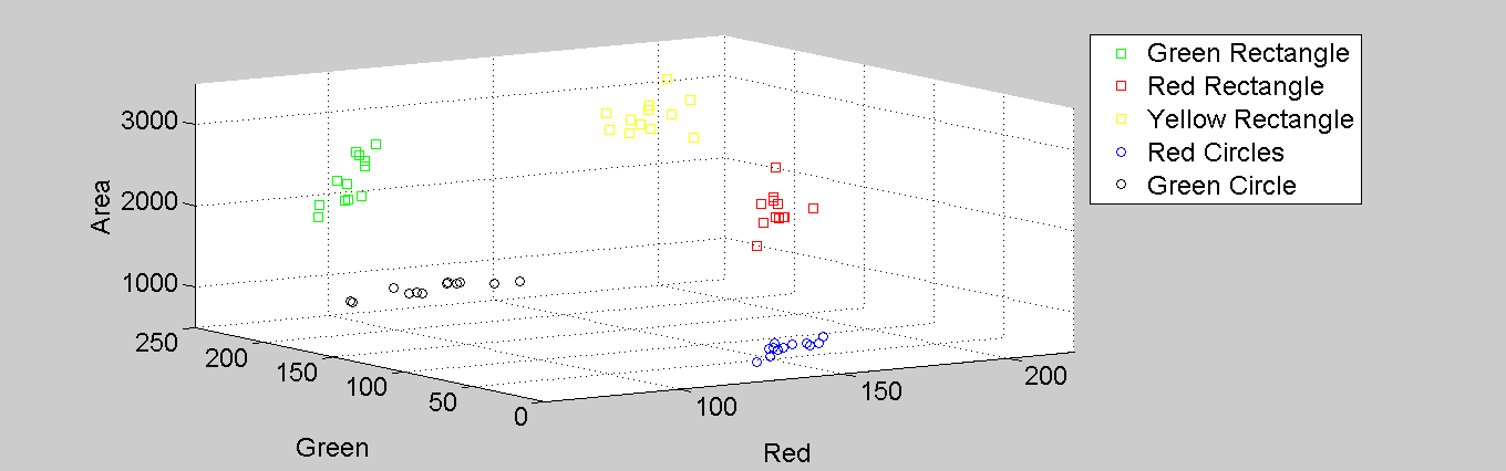
Figure 3. 3D scatter plot of the feature values
Shown in the Figure above is the 3D scatter plot of the three features chosen, as can be seen the groups are neatly separated. Now if we are to classify the remaining data set into their corresponding groups there are many methods that can be implemented, of which include the metric distance and linear discriminant analysis (LDA). Initially I will only be performing the metric distance method but if I would include the LDA latter on. For the metric distance method, one can perform either the K-nearest neighbor (k-nn) rule using euclidean distance or the Mahalanobis distance algorithm. For simplicity, I will be using the k-nn rule; in this method the euclidean distance was calculated between the texture values of the object to be classified, known as Instance, from all the training data set. The nearest k neighbors are taken as votes, the group with the most number of votes is where the instance will be classified into. k is preferably an odd numbered integer as to avoid a tie between vote. For this activity 16 samples represent each group, with 12 used as training data set, and 4 to be classified per group; k = 11.
Applying the method mentioned above, 18 out of the 20 data samples were correctly classified, giving an accuracy of 90%. But from where could have the error arisen from? Looking back into the features taken into account, it can be seen that the distance measurement is heavily dependable on the pixel area in terms of the magnitude of values. Thus to equally distribute the weights of each feature, these values has to be normalized. Doing this corrects the error observed earlier and a perfect classification is achieved.

Figure 4. Normalized feature values
For this activity I give myself a grade of 10 for completing the activity and performing the necessary applications.
No comments:
Post a Comment