Activity 5 - Area Estimation for Images with Defined Edges

For this activity we were to use Scilab in order to measure area via implementation of Green's Theorem. Recall that Green's Theorem allows an area integral to be related to a line integral. Given a region R bounded by a closed curve, composed of  Nb points arranged counterclockwise, we can estimate the area of the bounded surface based on the curve coordinates, stated as: 

we will be using binary images for the most part of the activity and later on move on to colored images. 

Recalling that from Activity 2, we were tasked with creating with creating binary images of a square and a circular aperture. In this activity, I will be reusing them to test the accuracy of the available edge detection methods available in Scilab. 

Shown in Figure 1 are two 300x300 binary image containing a 150x150 square and a circular aperture with radius = 45pixels. In applying the edge() function, there are three possible methods available; sobel, prewitt, and canny. As we can see from Figure 2, sobel and prewitt were able to detect the corner and the contour of the square, respectively, while the canny method was not able to detect anything. As such I will be using prewitt and sobel for the remainder of the activity.

Figure 1. 300x300 image with (Left) 150x150 square aperture; (Right) Circular aperture with radius = 45 pixels

Figure 2. Application of Edge detection methods: (Top and Bottom Left) Prewitt; (Top and Bottom Middle) Sobel: (Top and Bottom Right) Canny

Using find(), the edge coordinates along the x-axis and the y-axis were determined from the processed image. With the coordinates known, the center was shifted to the origin, as is the requirement needed for the equation to work.

[y,x] = find(E); //determine edge coordinates

//shift center to origin
x_unsort = x - mean(x);
y_unsort = y - mean(y);

What's left to do is to assured that the coordinates are arranged according to their position along the boundary of the object. The coordinates were thus represented in cylindrical space and sorting was implemented based on angle. For the ange conversion the atand() function was used, which mapped the coordinates along [-180,180]. For the sorting, gsort() function was used which returns a sorted array along with the original indices, which was used to sort the corresponding [x,y] coordinates.

//sort coordinates in counter-clockwise order
theta_unsort = atand(y_unsort,x_unsort);
[theta_sort,order] = gsort(theta_unsort);

L = length(x);

//sort x and y coordinates according to theta
x_sort = []; y_sort = [];
for i = 1: L
    x_sort = [x_sort, x_unsort(order(i))];
    y_sort = [y_sort, y_unsort(order(i))];
end

Area calculation was then applied based on Green's theorem.

//area calculations
Area = 0;
for i = 1: L
    if i == l then
        Area = Area + (x_sort(i)*y_sort(1) - y_sort(i)*x_sort(1));
    else
        Area = Area + (x_sort(i)*y_sort(i+1) - y_sort(i)*x_sort(i+1));
    end
end

Area = abs(0.5*Area)

The abs() function was used in the equation because the codes gives a negative value of Area. But this is not the only way to estimate the area of the apertures, another method known as Pixel counting can be used. In this case, I will be using pixel counting to count the number of 'white' pixels, the sum of which should be equal to the actual area of the object of interest. Pixel count method can also be used as a ground truth value in case the theoretical value does not match with the real value.

//set a groundtruth value
[void, pixelw] = size(find(A > 0));
gtruth = pixelw;

Table 1 shows the result after implementing the pixel count method and Green's Theorem based on the three mentioned edge detection technique.

Table 1. Area estimation results and percent error

For both the square and circle area estimation, it can be seen that the canny operator performed worst with a percent error of 100% which ensues due to the fact that it was not able to detect any part of the aperture boundary. This comes as a surprise since the canny edge method is supposed to be the standard edge detection method. Prewitt on the other hand exhibits the best result with the closest possible value to the pixel count method, with an error of 3 pixels for both aperture wrt pixel counting. Relating it to the theoretical value however shows that, like the pixel count value, it is farther away from the theoretical value compared to the Sobel operator. The error  that occurs is due to the synthesis of the circular aperture, it is not a perfect circle, what the code does is it approximates the boundary of the circle as close as possible as there are no fractional pixels. As shown in Figure 3, the boundary of the circle is not smooth and is actually pixelized, from this it is safe to assume that the Pixel counting and Prewitt-based application of Green's theorem has a more correct result compared to the Sobel-based approach.

Figure 3. Close up view of circular aperture boundary

Increasing the array size to 1000x1000, different area estimations were made for both square and circular apertures. In Figure 4 and 5, it can be seen that the for very small area estimation, both pixel counting and the Prewitt-based approach shows better results compared to the Sobel-based approach. But as the area of the apertures became larger, the error comparison between the three became insignificant, as shown in Tables 2 and 3. It is to note that for the circular aperture the Sobel-based approach was able to estimate the theoretical area of the circle more accurately than the two mentioned appraoches. However, the Prewitt-based approach has to closer approximation to the pixel counting method, which is used for the ground truth value. Also, reduction of the expected area was prominent throughout the synthesis of the circle and even in the smaller squares, which would have attributed to the error. Therefore, error should have been based from pixel counting rather than algebraic calculations.

Figure 4. Error maping for different Circular aperture area

Figure 5. Error mapping for different Square aperture areas

Table 2. Error calculation for circular aperture

Table 3. Error calculation for square aperture

Moving on to colored images, I took an image of the Pyramid of Giza from google maps by utilizing the Snipping tool. The area cover of the pyramid was first isolated using paint, shown in Figure 6 and the pixel to real world measurement was taken. For the image, every 119pixels corresponds to either 200ft or 50m. The image was then read using imread() and converted to grayscale using rgb2gray() function. Once this was done, all three edge detection techniques were used and area calculation via Green's theorem used. As shown in table 4, the Canny-approach was able to detect the edge of the pyramid outline, and the three edge detection method results varied minimally compared to each other. But the base length measurement of the pyramid varied based on the source, the one used in this activity was 693 ft, which can range from 693 - 765 ft. Using manual measurement of the pyramids base, it was estimated to have a base with a dimension of 435x436 pixels. Converting this to real world measurement, it can be seen that the Canny operator performed best followed by Prewitt and Sobel. Based from this, it can be said that the Canny operator is not applicable on binary images or arrays.

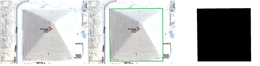
Figure 6. Pyramid base area islation; (Left) original image; (Middle) Distinguishing the edge of the pyramid; (Right) Isolation of the estimated Pyramid area cover

Table 4. Pyramid area and Error calculation based from source [1]

Table 5. Pyramid area and Error calculation based from manual estimation

In this activity, I believe I have performed beyond the requirements. Aside from meeting the set requirements I have also found error caused by the synthesis of the circle, made a comparison of the edge detection methods based on different area measurements and even discovered that the Canny operator does not work on purely binary values. I therefore would like to give myself a grade of 12.

Acknowledgements:
I would like to thank Alix for suggesting rgb2gray when gray_imread and im2gray would not work or function.

References:
[1]http://www.earthmatrix.com/great/pyramid.htm
[2]maps.google.com

Activity 4 - Image Types and Formats

In digital imaging there are four basics types which consist of:

• Binary images are characterized by two values, 0 or 1, which represent black or white, respectively. They are used in many processes since they are the most simplest to process. Though they also carry the least image information that they cannot be used all the time. However, they can be used on object identification, object orientation and text interpretation. A simple way in which to obtain a binary image is by thresholding a grayscale image.
  Shown below is an example of binary image of a binary number:

Figure 1. Binary image example [3]

Dimensions : 204 x 204

Width : 204 pixels

Height : 204 pixels

Horizontal Resolution : 96 dpi

Vertical Resolution : 96 dpi

Bit Depth : 24

Item type : jpeg file

• Grayscale images are images represented in shades of black and white, which range between 0 (black) and 255 (white) in numerical value, where in one pixel is one Byte. The need for a grayscale image is that it requires less information compared to a colored image. A gray image can be achieved in a colored image if rgb components in a pixel have the same values, but in a grayscale image only one pixel value is needed instead of three. Compared to a binary image, a grayscale image offers finer image details through the use of different gray tones.
  One such example of a grayscale image, which was derived from a true color image, is as shown below:

Figure 2. Grayscaled image

Dimensions : 600 x 337

Width : 600 pixels

Height : 337 pixels

Horizontal Resolution : 96 dpi

Vertical Resolution : 96 dpi

Bit Depth : 24

Item type : jpeg file

• True color images are images which are made up of three bands; one for each of the three primary colors. When the three are combined it is possible to replicate almost all of the colors, this is made possible because the human eye only has three color sensors, one for each of the primary colors. But since each pixel is composed of three bands, it is one of the heaviest images as can be seen on the details describing Figure 3.

Figure 3. True color image taken from an iPhone a year ago

Dimensions : 2048 x 1536                    Resolution unit: 2

Width : 2048 pixels                 Color Representation: sRGB

Height : 1536 pixels              Camera maker : Apple

Horizontal Resolution : 72 dpi              Camera Model : iPhone 3GS

Vertical Resolution : 72 dpi                           F-stop : f/2.8

Bit Depth : 24                          Exposure time: 1/15 sec

Item type : jpeg file              ISO speed : ISO-500

Focal length : 4 mm

• Indexed images are colored images whose colors are represented by numbers which denote the index of colors in a color map. Colored images makes use of a 24-bit color, but sometimes there is no need to make use of the full 24-bit range. Therefore indexing is used based on a variety of color palettes which can be composed of 8, 24 or 256 colors. The procedure is that the computer makes a list of the 256 most use color values, also called a color map or a color palette.In the past, indexed images were essential when computers were limited to only 256 colors, but up till present it is still used to save on bandwidth and storage space. One disadvantage though is that if an image is given a wrong color palette it is near to impossible to retrieve the original image.

Figure 4. Indexed image (Right) created using a color palette composed of 256 colors based from the original image (Left) [5]

Dimensions : 226 x 200

Width : 226 pixels

Height : 200 pixels

Bit Depth : 8

Item type : png file

There are many ways to identify image properties using Gimp, three of which include changing file format, histogram formation and image cropping, all of which I will implement upon the image shown in Figure 3 and 4.

Figure 5. Converted file (Left) and Cropped Image (Right)

Figure 6. Converted file (Left) and Cropped Image (Right)

Changing an images format is useful since each format offers its own advantages as will be discussed further own into the blog. Cropping on the other hand removes unnecessary details outside the region of interest and can even isolate features needed by the user. Lastly, a histogram plot of the image describes the color distribution along the image, which can be categorized into very dark, dark, medium, light and very light.

From the discussion earlier one can see that an indexed image, binary image and a grayscale image can be produced from a true color image. One has to simply manipulate the pixel values for each of the three color band to achieve this goal. Gimp, example offers a variety of tools with which one can perform the tasks mentioned. Shown in Figure 7 is another true color image used for this process. The image was originally of a larger size but was scaled down to 33% of its original value for easier handling.

Figure 7. True Color image of a Kite used in a ARRAS Fieldwork in the summer of 2012

Dimensions : 1006 x 754

Width : 1006 pixels

Height : 654 pixels

Bit Depth : 24

Item type : PNG

Size : 667kB

In gimp, one can convert this image into grayscale by right-clicking the image and selecting Image -> Mode  -> Grayscale. What happens is that Gimp varies the values along the RGB bands according to a set formula, one can actually perform the grayscale manually by using the channel mixer by going into Image-> Color-> Components -> Channel Mixer and define which percentage of the three bands/channels to use. But an easier way to is to go to Image -> Color -> Components -> Decompose, in this toolbox the user is offered a variety of ways in order to perform grayscale which allow image decomposition into CMYK, HSL, HSV, RGB and others. Decomposing the image into the RGB channel, results in three different grayscales as each channel can be represented in gray values. In Figure 10, note how the RGB channels differ from the default grayscale result. The variation is caused by the information that each channel contains. The red channel contains most of the luminance information as well as most of the noise. The green channel contains the least noise, while the blue channel contains shadow information and noise.

Figure 8. Selecting Grayscale tool

Figure 9. Selecting the Decompose tool

Figure 10. Grayscale result. (Top Left) Default Grayscale Result. Grayscale representation of the RGB channels: Red (Top Right), Green (Bottom Left), Blue (Bottom Right)

A binary image can be formed from a grayscale image or directly from the true color image. Gimp allows this by making use of the images histogram. Going into Image -> Color -> Threshold, a window opens containing a select region of the histogram and the image is converted into binary. Gimp gives a pixel value of 1 or white to the pixels falling into the highlighted histogram range while giving a pixel value of 0 otherwise.

Figure 11. Highlighted region in the histogram can be changed by the user although an autoselect function is available. (Left) Threshold toolbox. (Right) Resulting image derived from the upper left grayscale image in Figure 10.

Finally, the image can be indexed by going into Image -> Mode -> Indexed. Once clicked, a window appears in which the user defines how many colors should be present in the color palette. Using a color palette containing 256 colors, a quick glance shows that indexing did little to add changes in the image.

Figure 12. (Left) Indexed Toolbox window. (Right) Resulting Indexed Image 

Image can be divided into two formats:

• Lossy image compression, when applied, results in the lost of data and quality from the original file. In images this can be seen in the either the form of jagged edges or pixelation. But because the image is compressed, it is smaller in size compared to the original image. Examples of such an image format includes:
• GIF - Graphics Interchange format developed by CompuServe. These images are based on indexed images, which consists of a color palette of at most 256 colors. The compression of these images allow for fast transfer over a network though they lack the color range to be used for high-quality photos. This format is usually used for animated images and small icons. 
• JPEG - stands for "Joint Photographic Experts Group" named after the group which developed the format. This image format is not as limited to its color range like GIF which makes it highly used when compressing photographic images.

• Lossless image compression allows for the original data to be reconstructed from the compressed data. It is used when even a single pixel is crucial like in medical imaging, clipart and archiving important document. Examples include:
• PNG - Portable Networks Graphics was created as a replacement for GIF. It is the most used lossless image format and was designed for image transfer in the internet. Thus it is mostly RGB based (binary, grayscale, RGB[A], etc) and can support more than 8-bit RGB. It does not, however, support non-RGB color spaces.
• TIFF - Tagged Image File Format is used mostly by graphic artists and publishing industry and is controlled by the Adobe systems. It was developed in the mid-1980's to encouraged desktop scanner vendors to use a single format. TIFF began as a binary image but as scanners grew to support higher color palettes TIFF became able to support grayscale and, eventually, colored images. 
• MNG - Multiple-Image Network Graphics was released in 2001 as an animation version of PNG. 

Lastly, we were instructed to install SIVP in Scilab, but I have already installed the toolbox in the previous meeting so I just went ahead investigated the given functions.

imread and imshow, works hand in hand together. The former, loads an image from the specified file while the latter opens the image in different window. imwrite on the other hand saves the image to the specified format and is oriented as imwrite(data, filename.format)

gray_imread reads the image in the stated profile address into grayscale while im2bw converts an image into binary based on a threshold defined by the user. It is oriented as im2bw(name of image, threshold). This threashold ranges from 0 to 1, pixel values are normalized with respect to the maximum pixel value and those lower then the set threshold is given a pixel value of 0 while 1 otherwise.

histplot plots a histogram of the image according to the number of bins stated by the user. It assumes the form histplot( number of bins, data). Finally, imfinfo shows image information such as those shown in Figure 13.

In this activity, I have done everything that was asked and I felt that I even went beyond the requirement and thus I give myself a grade of 11.

References:

[1] http://homepages.inf.ed.ac.uk/rbf/CVonline/LOCAL_COPIES/OWENS/LECT2/node3.html
[2] http://homepages.inf.ed.ac.uk/rbf/HIPR2/gryimage.htm
[3] http://www.omomnia.com/room/binary-art/
[4]http://www.wookmark.com/image/131336/grayscale-pencils-grayscale-pencils-1920x1080-wallpaper-grayscale-wallpapers-free-desktop-wallpapers
[5]http://en.wikipedia.org/wiki/Indexed_color
[6]http://encyclopedia2.thefreedictionary.com/indexed+color
[7]http://www.gimp.org/tutorials/Color2BW/
[8]http://www.techterms.com/definition/gif
[9]http://www.techterms.com/definition/jpeg
[10]http://en.wikipedia.org/wiki/Portable_Network_Graphics
[11]http://en.wikipedia.org/wiki/TIFF
[12]http://www.libpng.org/pub/png/pngfaq.html#animation
[13]http://siptoolbox.sourceforge.net/doc/sip-0.7.0-reference/imfinfo.html

Activity 3 - Scilab Basics

Today we were tasked with implementing basic scilab plotting and imaging techniques. Scilab is basically an open source software for programming much like Matlab [1]. One example of a basic operation in scilab is plotting the graph of a sine wave.

 

Figure 1. Scilab code for sine wave

 

Figure 2. Resulting sine wave plot

Other basic commands include matrix addition (A + B), multiplication (A * B), and element-per-element multiplication (A .* B). Included in the manual is a code snipet which when implemented synthesizes an image of a circular aperture.

Figure 3. Code sniper for circular aperture with a radius of 0.9

Figure 4. Synthesized aperture from figure 3

Most of the code is pretty much self-explanatory, but of import are lines 5-7 which define the whole aperture itself. Line 5 makes use of the grid created in line 4. The grid which uses the Cartesian coordinate, uses the center pixel as the origin (learned this by experimenting with the snipet). Thus line 5 is actually an array of pixel distance measurement from the origin, assuming that the x- and y-axis range is from [-1, 1]. Line 6 constructs a matrix, A, using the same dimension as X and Y. Line 7 assigns the radius of the aperture, it can be of any arbitrary value but in this code I used 0.9. The radius can even be greater than 1 although the image parameters wouldn't allow the synthesized image to show the whole aperture.

With that done, we will now dwell on the tasks given for the activity, which are to synthesize:

• Centered Square Aperture
• sinusoid along the x-direction (corrugated proof)
• grating along the x-direction
• annulus
• circular aperture with graded transparency (gaussian transparency)

For the centered square aperture, it follows directly from the circular aperture, only line 5 is no longer needed.

Figure 5. Changed snippet from figure 3

Figure 6. Synthesized square aperture with side length 1.4 units

In line 6 all pixels encompassed with in the [-0.7, 0.7] range along the x- and y-axis are assigned with the value 1 creating a white square aperture. The addition of the abs() and '&' commands were used, they were not necessary but were helpful in making the code shorter. Also, instead of the grayplot(), imshow() was used. The addition of this command required the installation of SIP.

For the corrugated sine wave plot required the application of the sine wave function for the X matrix.

Figure 7. Code for corrugated sine wave, image parameters were enlarged for larger images

The only addition here is that the sinusoid was plotted using the grayplot() and the imshow() function. And it was surprising that they showed slightly different results. For the grayplot(), the wave was propagating along the x-axis, but the imshow() plot showed that the wave is propagating along the y-axis. But since the grayplot() had an additional grid and axis for reference, it should be exhibiting the correct behavior of the plot.

Figure 8. (Left) Plot from grayplot(); (Right) Plot from imshow()

One other possible way to plot this is by mesh() function [2](replace line 12 with mesh(A)), which will plot it in 3D.

Figure 8. 3D graph of the corrugated sine wave with f = 2

The grating can be extracted from the sine wave snippet, it only requires the implementation of the round() and abs(). Since the sine wave ranges from [-1,1], the round() function rounds of the values of the sinusoid matrix, making only Three values possible; -1,1 and 0. Then the abs() function ensures that the only value are 1 and 0. In theory, this should produce an equally spaced grating, but this does not seem to be the case and still baffles me up to this date.

Figure 9. Grating code snipped

Figure 10. Generated grating with f = 9. This plotted using imshow() and flipped in order 

to represent the grating correctly as the grayplot() does not show a real grating.

Figure 11. Generated 3D grating with f = 5. (Left) Front view; (Right) top right view

The annular is simply a circular aperture with a limited range, there are three ways I can think of in order to implement this but the shortest would make use of the '&' command. Returning to figure 3  line 5, one only needs to change find(r < 0.9) with find(r > 0.3 & r < 0.7), thus creating the annular. The thickness of the ring can be modified by changing the two arbitrary values.

Figure 12. Generated annular ring with r1 = 0.3 and r2 = 0.7

Lastly, the circular aperture was generated by creating a plot of a gaussian distribution in grayscale and then applying the circular aperture. The gaussian function I used was googles using the keyword "2D gaussian function" [3].

Figure 13. Snippet with gaussian transparency

Figure 14. Generated gaussian transparency

Earlier I said earlier that there were two other ways of synthesizing the annular ring. Referring to Figure 15, if we use the image produced from matrix A and B or matrix A and C and perform matrix element-per-element multiplication or subtraction, respectively then we will arrive with the same image shown in Figure 12.

Figure 15. Generated circular aperture. (Left) r = 0.7. (Mddle) r = 0.3. (Right) r = 0.3. Either A.*B or A - C will result in Figure 12.

In this experiment, I will give myself a grade of 10 since I believe that I have met and accomplished all the requirements for the activity. I would like to thank Chester Balingit for helping me install SIP, I would to thank James Vance for the motivational support, Nestor for being funny and Alix for assuring me that what I am doing is correct.

References:
[1]https://www.scilab.org/scilab/about
[2]http://help.scilab.org/docs/5.3.3/en_US/mesh.html
[3]http://www.site.uottawa.ca/~edubois/courses/CEG4311/plotting_2D.pdf

Activity 2 - Digital Scanning

Today we were tasked with bringing a digital copy of any hand drawn plot from any journal from the nearby CS library. I took a graph from Effect of Laser-induced collisions on chemical reactions by Sister Kathleen Duffy, but the scanning process left the right-edge of the page blurred and distorted. It wasn't much of a bother until the activity tasks were given for the day.

We were to reproduce the graph using any spreadsheet by extracting pixel coordinates based from the tick marks. Since the graph I had were blurred, this would cause error during initial measurements. It was just my luck that the girl scout next door and my classmate, Abigail Jayin, had a spare graph about Electron density profiles.

Figure 1. Scanned copy of the Electron density profile [1]

The first step was to calculate the conversion equation between pixel coordinates and the graph's x- and y- coordinates. In order to obtain the pixel-to-physical value ratio, paint was used, as shown in Figures 2 and 3. The crop tool in GIMP was also utilized in order to isolate and align the graph, removing the need for reference points and allowing direct extraction of values. 

Figure 2. Using paint to measure x-axis pixel location conversion

Figure 3. Using paint to measure x-axis pixel location conversion

The x-axis conversion was easily acquired; 127 pixels/cm. The y-axis conversion proved to be more troublesome as it arranged its physical values in logarithmic space. What had to be done initially was the same for the x-axis. Direct conversion shows that for every 792 pixels corresponds to 1 unit in the logarithmic space. In order to perform this, the pixel coordinate has to be flipped since the origin in an image starts at the upper left. The y-pixel coordinates are then to be converted into logarithmic coordinates and the results used as exponents with a base of 10. Final results are then to be multiplied by 10 of the ninth power, shifting the results into the range of graph. Thus the determined proper pixel to physical value conversion equation are as follow:

• x = xp/65

• y = 10^((1589-yp)/792)*(10^9))

Where x and y are the physical variable value and xp and yp are the pixel location. In order to acquire pixel coordinates along the graph more accurately, grids were introduced unto the digital graph to use as a guide. Taking in 20 pixel coordinates from the lower graph, they were converted using the two equations mentioned and plotted atop the original graph for comparison. As can be seen in Figure 4. Results show that the points were plotted accurately as the points overlaps with the original points.

 It is noticeable that some of the plotted coordinates strays from the original by some marginal value. This could have been brought about by improper measurement of pixel location. Another probable cause would have been the graph itself. Recall that the graph is hand drawn and is subjected to human error. Analyzing the graph it can be seen that it is not entirely perpendicular with respect to the image borders in Figure 1. The cropped image of the graph was already straightened using gimp in order to untilt the graph or at least minimize tilting. This, however, seemed unavoidable as can be seen in Figure 4. Although unnoticeable with a white background, close up the edge of the plot is not perpendicular to the base of the image. With the grid lines for the experimental graph present though, the misalignment of the graph is more prominent. The implementation of how the page was scanned could have also contributed to the skewed edges, as parts of the pages could have been more elevated during the scan. Returning to Figure 4, the left part of the graph is tilted while the right edge is aligned with the edge of the image. Yet overall, the resulting plot is satisfactory enough with a relatively small deviation.

Figure 4. Pixel-coordinate conversion plot. The y-axis was also represented in logarithmic scale.

I would like to give myself a grade of 11 overall as it seems that I met all of the requirements or may have even exceeded it with the added difficulty for the logarithmic conversion. I would also like to acknowledge Abigail Jayin who is the generous source of my graph, Chester Balingit for scanning the graph, and Alix Santos for guiding me.

Sources:

[1] Effect of Laser-induced collisions on chemical reactions, Sister Kathleen Duffy, Proceedings of the 4th National Physics Congress, 1985