Activity 3 - Scilab Basics

Today we were tasked with implementing basic scilab plotting and imaging techniques. Scilab is basically an open source software for programming much like Matlab [1]. One example of a basic operation in scilab is plotting the graph of a sine wave.

 

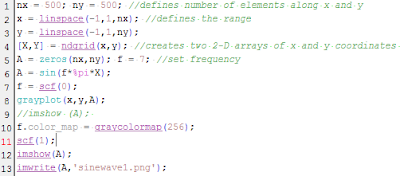
Figure 1. Scilab code for sine wave

 

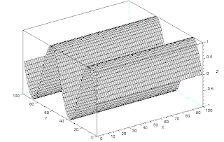
Figure 2. Resulting sine wave plot

Other basic commands include matrix addition (A + B), multiplication (A * B), and element-per-element multiplication (A .* B). Included in the manual is a code snipet which when implemented synthesizes an image of a circular aperture.

Figure 3. Code sniper for circular aperture with a radius of 0.9

Figure 4. Synthesized aperture from figure 3

Most of the code is pretty much self-explanatory, but of import are lines 5-7 which define the whole aperture itself. Line 5 makes use of the grid created in line 4. The grid which uses the Cartesian coordinate, uses the center pixel as the origin (learned this by experimenting with the snipet). Thus line 5 is actually an array of pixel distance measurement from the origin, assuming that the x- and y-axis range is from [-1, 1]. Line 6 constructs a matrix, A, using the same dimension as X and Y. Line 7 assigns the radius of the aperture, it can be of any arbitrary value but in this code I used 0.9. The radius can even be greater than 1 although the image parameters wouldn't allow the synthesized image to show the whole aperture.

With that done, we will now dwell on the tasks given for the activity, which are to synthesize:

• Centered Square Aperture
• sinusoid along the x-direction (corrugated proof)
• grating along the x-direction
• annulus
• circular aperture with graded transparency (gaussian transparency)

For the centered square aperture, it follows directly from the circular aperture, only line 5 is no longer needed.

Figure 5. Changed snippet from figure 3

Figure 6. Synthesized square aperture with side length 1.4 units

In line 6 all pixels encompassed with in the [-0.7, 0.7] range along the x- and y-axis are assigned with the value 1 creating a white square aperture. The addition of the abs() and '&' commands were used, they were not necessary but were helpful in making the code shorter. Also, instead of the grayplot(), imshow() was used. The addition of this command required the installation of SIP.

For the corrugated sine wave plot required the application of the sine wave function for the X matrix.

Figure 7. Code for corrugated sine wave, image parameters were enlarged for larger images

The only addition here is that the sinusoid was plotted using the grayplot() and the imshow() function. And it was surprising that they showed slightly different results. For the grayplot(), the wave was propagating along the x-axis, but the imshow() plot showed that the wave is propagating along the y-axis. But since the grayplot() had an additional grid and axis for reference, it should be exhibiting the correct behavior of the plot.

Figure 8. (Left) Plot from grayplot(); (Right) Plot from imshow()

One other possible way to plot this is by mesh() function [2](replace line 12 with mesh(A)), which will plot it in 3D.

Figure 8. 3D graph of the corrugated sine wave with f = 2

The grating can be extracted from the sine wave snippet, it only requires the implementation of the round() and abs(). Since the sine wave ranges from [-1,1], the round() function rounds of the values of the sinusoid matrix, making only Three values possible; -1,1 and 0. Then the abs() function ensures that the only value are 1 and 0. In theory, this should produce an equally spaced grating, but this does not seem to be the case and still baffles me up to this date.

Figure 9. Grating code snipped

Figure 10. Generated grating with f = 9. This plotted using imshow() and flipped in order 

to represent the grating correctly as the grayplot() does not show a real grating.

Figure 11. Generated 3D grating with f = 5. (Left) Front view; (Right) top right view

The annular is simply a circular aperture with a limited range, there are three ways I can think of in order to implement this but the shortest would make use of the '&' command. Returning to figure 3  line 5, one only needs to change find(r < 0.9) with find(r > 0.3 & r < 0.7), thus creating the annular. The thickness of the ring can be modified by changing the two arbitrary values.

Figure 12. Generated annular ring with r1 = 0.3 and r2 = 0.7

Lastly, the circular aperture was generated by creating a plot of a gaussian distribution in grayscale and then applying the circular aperture. The gaussian function I used was googles using the keyword "2D gaussian function" [3].

Figure 13. Snippet with gaussian transparency

Figure 14. Generated gaussian transparency

Earlier I said earlier that there were two other ways of synthesizing the annular ring. Referring to Figure 15, if we use the image produced from matrix A and B or matrix A and C and perform matrix element-per-element multiplication or subtraction, respectively then we will arrive with the same image shown in Figure 12.

Figure 15. Generated circular aperture. (Left) r = 0.7. (Mddle) r = 0.3. (Right) r = 0.3. Either A.*B or A - C will result in Figure 12.

In this experiment, I will give myself a grade of 10 since I believe that I have met and accomplished all the requirements for the activity. I would like to thank Chester Balingit for helping me install SIP, I would to thank James Vance for the motivational support, Nestor for being funny and Alix for assuring me that what I am doing is correct.

References:
[1]https://www.scilab.org/scilab/about
[2]http://help.scilab.org/docs/5.3.3/en_US/mesh.html
[3]http://www.site.uottawa.ca/~edubois/courses/CEG4311/plotting_2D.pdf