Activity 10 - Morphological Operation

Morphology refers to shape or structure. In image processing, morphological operations are usually performed on binary images, where the data formation of 1's are of interest, so as to improve the image or to extract information, i.e. Isolation and Detection of Spectral line. Thus by this notion, morphological operation affects the shape of the image. In implementing Morphological operations, it is essential to understand set theory.

If assume A to be a set in 2D interger space, and let a be an element of A, then this is represented as,

and if we assume an element b  set B which is not found in set A then

 If however we want to denote A as a subset of B then

which denotes that all elements of A can be found in B but not otherwise. 

Set operations on the other hand include union, which is a set containing all elements contained in the two sets related to the operation, denoted by:

while an intersection denotes a set that contains identical elements between two sets denoted by:

If, however, the two sets are mutually exclusive or that they have no common elements, then the resulting intersection between the two would be result in a null set, shown as:

A complement of A is a set which contains all elements not present in A is denoted as:

the last two set operation are reflection, or flipping the set, and translation, denoted as:

respectively.

In morphological operation, two basic techniques are the dilation and erosion. Dilation is denoted as:

which denotes that the operation is a dilation of A by B. Mathematically, the operation is read such that the structuring element, B, is reflected and will involve all z's such that the intersection of A and the translation of the reflected B does not result in a null set. Thus the effect of Dilation either expands or elongates the image. Erosion on the other hand is denoted by:

which reads as the erosion of A by B. The operation involves all z's such that B translated by z is contained in A or will result such that B will become a subset of A.

Dilation and Erosion can thus be performed manually. In this activity Dilation and Erosion were performed on the following images:

Figure 1. (Leftmost) 5x5 Square (Middle Left) Right Triangle with base = 4 and height = 3 (Middle Right) 10x10 Hollow square with a thickness of 2 pixels and (Rightmost) Plus sign 5 pixels across with 1 pixel thickness

 Using the following structuring elements:

Figure 2. (Leftmost) 2x2 Square (Middle Left) 2x1, (Middle) 1x2 (Middle Right) Plus sign 3 pixels across (Rightmost) 2x2 Diagonal

Implementing each and every Structure element per image, manually through Excel and automatically through Scilab, we compare the results.

 

Figure 3. Solid Square (Top) Manual Dilation and Erosion. (Bottom) Through Scilab

Figure 4. Triangle (Top) Manual Dilation and Erosion. (Bottom) Through Scilab

Figure 5. Hollow Square (Top) Manual Dilation and Erosion. (Bottom) Through Scilab

Figure 5. Plus (Top) Manual Dilation and Erosion. (Bottom) Through Scilab

As can be seen, the results are exact for the application of Erosion and differ for the Dilation. In my perspective, it seems that the dilation of Scilab did not apply reflection during dilation and as such the difference observed above. 

I would like to apologize for the late submission which was caused by faulty internet connection.

Reference:

[1] M. Soriano. "Morphological Operations". Applied Physics 186 2013. University of the Philippines

Activity 8 - Enhancement in the Frequency Domain

This activity is focused on noise cancellation or removal in images. Main concepts to be used in this activity focuses on application of Fourier Transform via FFT in 2D space and convolution, both of which was discussed in Activity 7. But before we go into noise cancellation, we will first look into various insights into convolution and FFT.

First we synthesize a 200x200 binary image of various shapes, as shown in the top row of Figure 1. Now the first image from the left, shows two equally spaced dots, but mathematically this can be viewed as two Dirac deltas, and as such we can see that the Fourier of such an image results in a sinusoid. Though its sinusoidal pattern is not as clear as plotting it in 3D, the varying intensity of the plot should suffice in supporting the statement. Increasing the distance between the two dots would result in a higher frequency sinusoid, as would decreasing the pixel distance result in a lower frequency sinusoid. From the previous Activity it was shown that by applying fft2() to an image would give of its representation in frequency space but applying it again would revert it back to the original image. Also recall that FT represents data into its frequency components, now assuming that the two equally spaced dots represent the frequency of a sinusoidal function then applying fft2() would result in an image representing such a function, as was shown. 

Figure 1.(Top row) Synthesized images of equally spaced dots, circles, squares and Gaussians. (Bottom Row) Resulting Fourier Transform  

The second image is that of two equally spaced circles, which is a convolution of the previous spaced dirac delta and a circle. As such the resulting transform of the two should be a element-per-element multiplication of the transforms of the two images as shown in Figure 1. The output is that of a sombrero function superimposed upon a sinusoidal function which are the transform of a circle and of two Dirac deltas, respectively. This concept can also be observed in the other two images in Figure 1. The third and fourth top row image shows the convolution of a square and of a Gaussian to two Dirac deltas, respectively. Since the transform of a square is a sinc function and the transform of a Gaussian is a Gaussian the output is as shown in Figure 1. Note however that increasing the variance of the Gaussian in the input will lead to a smaller Gaussian in the frequency space and decreasing variance will result in the opposite.

The process in which the previous images can be explained by performing the following. Synthesizing 10 Diracs randomly distributed along a 200x200 black image, and a random pattern, as shown in Figure 2. Taking the transforms of the two images and performing element-by-element multiplication of the results then applying fft2() to the product would result to the image shown in Figure 3. As can be seen the pattern is superimposed on each dot from the earlier image. In the same manner, one can replicate the images in Figure 1.

Figure 2.(Left) Randomly placed Dirac Deltas. (Right) Diamond Pattern

Figure 3. Resulting Fourier Convolution of the images in Figure 2. Image was flipped for comparison.

Now implementing fft2() to equally spaced vertical lines, shown in Figure 4, will result to fringes, also shown in Figure 4. The Fourier transform sees that image as an array of equally spaced Dirac Deltas or Dirac Delta train, applying fft2() to such an array would result in a Dirac Delta train with a spacing, 1/T, equal to the inverse of the spacing in the spatial domain, T. Thus as shown in Figure 4, as the spacing between the dirac train increases, the spacing between the fringes lessens.

Figure 4. (Top Row) Equally spaced dirac trains. (Bottom Row) Fringe Patterns.

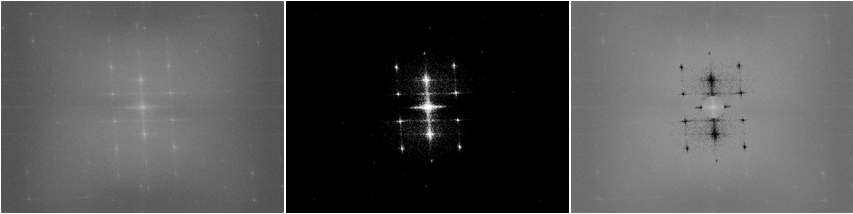
Returning to noise cancelling, noise can be defined as unwanted signal that is considered to be spurious and extraneous information, and is usually a by-product of how the image was captured. In Figure 5 for example, the image exhibits equally spaced vertical lines similar to those of Figure 4. These are the result of digitally stitching of 'framelets' in order to form the image. Analyzing the transform of the image, the fringe pattern which was shown earlier, can also be observed both horizontally and vertically. A mask or a filter was thus synthesized in order to remove the noise, which consisted of pattern much like a crosshair since the middle part of the transform has to be kept the same since low frequency is usually the domain of important image data. After performing element-per-element multiplication between the mask and the FT of the image, performing fft2() to the result gives of a filtered image without the prevalent noise observed in Figure 5.

Figure 5. Moon image with equally spaced vertical lines [2]

Figure 6. (Left) Fourier Transform of Figure 5. (Middle) Mask. (Right) Superimposed masked on FT of the Moon image

Figure 7. Filtered image after applying mask

Another way of performing this is by measuring the pixel distance between each vertical line, then from that replicate the pattern of the vertical lines. Take the transform of the pattern perform element-per-element division from the transform of the image in Figure 5, the resulting image should give an output similar or identical to that of Figure 7.

The last image to be to be subjected to noise cancellation is, shown in Figure 8, a painting by Dr. Vincent Daria. Shown in Figure 9 is the transform of the image. Since no pattern can be generated quickly, a quick way to create a mask is to threshold the transform and convert it to binary. Now getting the negative of the binary and superimposing a circle to the center and the mask for the image is complete. The result is shown in Figure 10.

Figure 8. Oil Painting by Dr. Vincent Daria

Figure 9. (Left) FT of Figure 8. (Middle) FT after applying the threshold. (Right) Filtered FT

Figure 10. Filtered image from Figure 8

In this activity I give myself a grade of 10, for completing the task and for being able to comprehend and explain the performed tasks.

Reference:
[1] M. Soriano. "Enhancement in the Frequency Domain". Applied Physics 186 2013. University of the Philippines.

[2] lpi.usra.edu. "Apollo 11 Mission". Accessed on July 30, 2013.  http://www.lpi.usra.edu/publications/slidesets/apollolanding/ApolloLanding/slide_05.html

[3] http://en.wikipedia.org/wiki/Image_noise

Activity 9 - Color Image Segmentation

Image segmentation, by definition and by my experience after performing this activity, is the partitioning of images into parts for the purpose of identifying objects and/or other relevant information. Segmentation can also be done by thresholding, as shown in Activity 4, but sometimes this does not suffice. Thus in this activity color image segmentation will be performed. 

As color can be perceived in different shades and brightness, it would be efficient to represent colors in terms of chromaticity and brightness. One such space is known as the normalized chromaticity coordinates. As the name suggests, each pixel coordinate is normalized:

where R, G, and B are the matrix representing the red, green, and blue channel of the image, respectively. Here I = R + G + B and r+g+b = 1, where r,g and b can only have values from 0 to 1 and b is independent of r and g. Thus we can represent chromaticity in terms of r and g and brightness is given by I. In the NCC space; where r and g is zero, corresponds to the coordinate, blue, while where r = 1 and g = 1 corresponds to pure red and green, respectively.

Figure 1. NCC model

There are two techniques in which the image can be segmented, either parametric or non-parametric probability distribution estimation.

In Parametric probability distribution estimation (PPDE), as is in non-parametric, we first select from the image a region which belongs to a color distribution of interest (CDOI). In the image shown in Figure 2, that would be the red coloration in the kite. From this region of interest (ROI) we can compute the probability of each individual pixel in the image of being part of the color distribution of interest. 

Figure 2. Image taken of a Kite during an Arras Fieldwork

Figure 3. ROI

Since NCC is represented in r and g, the joint probability from each channel is calculated. Thus for each channel a Gaussian distribution is assumed, represented as:

where µ  and σ are the mean and standard deviation derived from the ROI, and r and g are pixel coordinates from the image. Thus by taking joint probability per pixel, the application of PPDE to the image is complete.

Figure 4. Image Color Segmentation Result after application of PPDE

In Non-Parametric probability distribution estimation (NPPDE) histogram backprojection is used. This method is similar to that of Activity 6 except in this activity this is performed in 2D. After normalizing the r and g channels we can compute its histogram by implementing this code:

BINS = 32;

rint = round( r*(BINS-1) + 1);

gint = round (g*(BINS-1) + 1);

colors = gint(:) + (rint(:)-1)*BINS;

hist = zeros(BINS,BINS);

for row = 1:BINS

    for col = 1:(BINS-row+1)

        hist(row,col) = length( find(colors==( ((col + (row-1)*BINS)))));

    end;

end;

scf(2);

imshow(hist,[]);

where hist coordinates are given by rint and gint given as (rint, gint) but since images are represented in row and column, the rint coordinates would be located along the y-axis and the gint coordinates along the x-axis while the origin is now located at the top left corner. As shown in Figure 5, the resulting histogram of the ROI from Figure 3 agrees with the NCC model.

Figure 5. Comparison of NCC model and histogram of Figure 3

Thus by converting each pixel from Figure 2 into rint and gint coordinates and performing histogram backprojection, the image is segmented.

Figure 6. Image Color Segmentation Result after application of NPPDE

Comparing the two results,

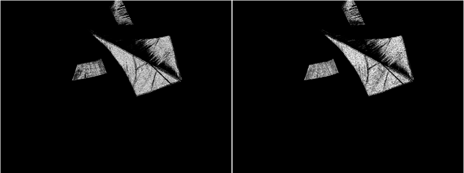
Figure 7. Comparison of results PPDE (left) and NPPDE (right)

we can see that NPPDE detects more of the CDOI compared to PPDE, which neglected most of the pixels in the shadowy region. Thus overall, NPPDE has a faster and less complicated application and a more accurate result compared to PPDE.

In this activity I give myself a grade of 10 for being able to implement the tasks given and for being able to understand the steps involved.

Acknowledgement

I would like to thank Anjali Tarun for teaching me what was wrong in my NPDDE code.

Reference:

[1] M. Soriano. "Color Image Segmentation" Applied Physics 186 2013. University of the Philippines

Activity 7 - Fourier Transform Model of Image Transformation

Fourier transform (FT) is a linear transform which converts a signal from spatial domain into frequency domain. In image processing, FT is mainly used in decomposition of an image into its sine and cosine components. Thus each point in the resulting Fourier image represents a particular frequency contained in the spatial domain. Such is the usefulness of FT that it can determine the relative strength of any periodic data and show periodicity in any input data [1]. The FT of a 2D-image f(x,y) is given by [2]:

One constraint of applying applying FT, however, is computation time, in that at large data input's will take a considerable time to compute [3]. Which is why in 1965, Colley and Tukey developed an algorithm, termed the Fast Fourier Transform (FFT), as a fast and efficient implementation of FT [2]. In the software in which this activity was performed, Scilab 5.4.1, the FFT functions are fft() for 1D signals and fft2() for 2D signals, which is where grayscale images fall under.

In order to test the performance of fft2(), an 128x128 image of a white circle with a black background was synthesized. If we consider an image array to be sectioned in four quadrants, then applying fft2() will interchange the results along the diagonals. The orientation of the original quadrants can be recovered by applying fftshift(), as shown in Figure 1.

Figure 1. (Top Row) Input Image. (Middle Row) Output image after applying FFT2 and (Bottom Row) after applying fftshift. From left to right column; radius (r) = 5, 7, 10, 15 and 20 pixels.

From Figure 1, circles of varying radii were synthesize, ranging from 5 to 20 pixels. The images were converted to double before applying fft2(). fftshift() was them applied to the output to return the quadrants to their original orientation. Based from the results, it can be observed that as the radius of the synthesized aperture increases, the radius of the resulting ring formations in Fourier space decreases. Yet as this occurs, the ring formations steadily become less broken. The broken feature of the ring formations can be attributed to the rasterization of the circle as discussed in Activity 5. As the circle is represented digitally, the smaller the image and the smaller the circle, the more is the circle approximated, resulting in an imperfect circle [4]. In essence, the output is actually a sombrero function [4]. The sombrero function (jinc(t)) can be represented as a Bessel function of the first kind. As Bessel function are analogous to sines, it thus follows that the sombrero function is analogous to the sinc function [5].

where J1 is the Bessel function of the first kind. The distance of the first dark ring from the middle is given by [4]:

where N is the pixel length of the image, N = 128, and r is the radius of the circle. Thus for the 20 pixel radius circle, the distance of the first dark ring to the center pixel is given by x1 = 0.66*128/20 = 4 pixels.

Next an binary image of the letter A was created using paint, to observe the quadrant interchange discussed earlier. This was not shown through the binary image of the circle since the inversion of a circle will still result in a circle.

Figure 2. (a) Input Image, Leftmost. (b) Fourier of (a), Inner Left. (c) After applying fftshift() to (b), Middle.

(d) After applying fft2() to (c). (e) Double application of fft2() to (a) 

As can be seen in Figure 2, applying fft2() to the image, interchanges the quadrants or inverts the image, but if fftshift() is applied, the quadrants is reverted back to their original position.

In utilizing FFT for image processing, there are three concepts which will be tackled in this activity; convolution, correlation, and edge detection. Convolution is a linear operation which follows the convolution theorem:

where H, F and G are the transforms of h, f and g, respectively. Convolution can be defined as the imprinting one function unto the other such that the output resembles both functions though not completely. In 2D, the equation for convolution is given as [2]:

In Scilab, this can be done by element-per-element multiplication of two images in Fourier space. Thus another text image was synthesized using Paint as shown in Figure 3.

Figure 3. Text image 

fft2() was then applied to the image. The image was then convolved with the circular apertures shown in Figure 1. Recall that the FT merely translates the signal into frequency space, thus if the quadrants are in there natural orientation, then the fft2() represents the signal in 2D Cartesian coordinates.Thus center values along the image are low frequency, while those nearer the edge are high frequency data. By applying convolution via element-per-element multiplication with a binary circular aperture, we are applying a low-pass filter through the Fourier space, or we are applying a mask. Which is why it can be seen in Figure 4, that as the radius of the aperture increases, the more clearer is the text since more feature data is left unfiltered.

Figure 4. (Top Row) Mask applied. (Bottom Row) Resulting image after convolution.

Image is inverted due to application of fft2() twice and fftshift() once.

Correlation is given by the equation [2] in 2D space:

where p denotes the correlation of the two functions f  and g, which denotes the degree of similarity between the two. Thus correlation is mostly used in template matching and pattern recognition. In Scilab, this was implemented by applying fft2() to the text image shown in Figure 5 and the letter texts shown in Figure 6. Element-per-element multiplication between the transform of the letter text and the conjugate transform of the sentence text was performed. The transform of the product was then taken. As shown in Figure 6, results show high correlation between the two images, although clarity varies. It can be observed that the output image is sharper as the font size difference between the two lessens, thus the image is heavily blurred when correlation is taken from the large font text.

Figure 4. Text image  

Figure 5. Letter text of varying font size (Top row).  Resulting correlation (Bottom Row) 

Due to the mechanics behind edge detection, we can assume that it is a template matching technique. As such, this can be done by convolution of a 3x3 pattern to the image of interest. Shown in Figure 7 are the different patterns used in the experiment, but, as can be seen, the dot patter exhibited the best result. This is because the dot pattern showed is independent of direction, as we can see in the horizontal and vertical pattern. To discuss further, if the pattern is centered inside the text or outside, will incur a value of zero due to the summation of the values. If the pattern is centered along the edge of the text, then it will incur a positive value an automatic white. For the other patterns however, like the horizontal patter, if it was centered along the vertical edge, it will result in a value of zero, due the distribution of the values.

Figure 6. (Top Row) Patters, from left to right, horizontal, vertical, diagonal, dot. (Bottom Row) Result after convolving pattern with image in Figure 3 in Fourier space, with the images flipped for comparison.  

In this activity I give myself a grade of 10, because I have performed all tasks completely with an understanding and explanation of what was done.  

Activity 6 - Enhancement by Histogram Manipulation

Images taken from environments too dim or too bright has a histogram which is more likely to be one sided. That is why in this activity we were tasked with enhancing an image via Histogram manipulation. Thus in this activity we will be applying a histogram manipulation technique known as backprojection.

The histogram of the image in grayscale is taken and normalized with the number of pixels present within the image. This normalized histogram is known as the probability distribution function (PDF). Taking the cumulative sum of the histogram, we have the cumulative distribution function (CDF) of the image. We then project the CDF of the image to a desired CDF.

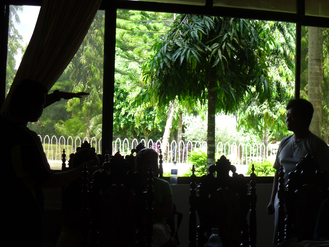
Doing this in Scilab, the image of interest, shown in Figure 1, is converted into grayscale using the rgb2gray() function. At first glance, one can see that there are two people having a discussion within the image with a third sitting between them. Though due to the bright background, the camera was not able to exhibit details pertaining to the subjects except their silhouette.

Figure 1. Image taken during a fieldwork in Samal

Details:

Dimension - 1280x960

Resolution - 96 dpi

Bit Depth - 24

Figure 2. Grayscale image of the image

The histogram of the grayscale is taken using imhist(), and normalized based from the minimum and maximum  grayscale values to get the PDF.

[count, null] = imhist(gscale, 255);
counts = (counts - min(counts)/max(counts);

Figure 3. Normalized histogram of the Image

where in count is the array containing the histogram and eventually becomes the PDF of the image, gscale is the name of the grayscale of the image and 255 is the number of bins I want for the histogram. In this condition, pixel distribution per grayscale value is accounted for. As one can observe, the image shown is very dim due since the objects of interest were against the light. This is reflected in the histogram of the image as shown in Figure 3. From Activity 4 there were five proposed areas in the histogram; very dark, dark, neutral, bright, and very bright. From the histogram, it can be seen that the pixels are tightly spread in the  very dark category of the histogram. Taking the CDF of the image by applying the cumsum() function to counts and normalizing the values results to the plot seen in Figure 4..

Figure 4. CDF of the Image

What we want is an images with its pixel distribution centered about the neutral region of the histogram. This will bring out the details left out by the camera in order to adjust to the abundance of light. Thus a normalized 2D-Gaussian function was used as the ideal PDF for the image. 

where sigma is the standard deviation, and a is the mean. For this image, I used a = 128 and sigma = 30. Normalizing the Gaussian function, I now have constructed the ideal PDF of my image, shown in Figure 5, followed by the ideal CDF.

Figure 5. Ideal PDF, sigma = 30 and centered at 128

Performing backtracing, I simply called out each corresponding CDF value per gray level from the image and  compared it with the gray level from the ideal with the same CDF value. I replaced the image gray level with that of the ideal and processed the image.

for i = 1:length(gvalue)
    [j] = find(CDFideal <= csum(i));
    imp_im(find(gscale == gvalue(i))) = gvalue(j($))
end

where, imp_im is a copy of the gscale matrix I mention earlier and gvalue is the range of gray level values. At first I was implementing imp_im as a 2D matrix of zeros, but for some apparent reason the code won't work properly with this. I even tried creating imp_im as a 3D matrix of zeros and then converting it to grayscale using rgb2gray but the code still won't work. It was only when I implemented imp_im as a copy of gscale that I was finally able to produce the processed image shown in Figure 7.

Figure 6. Ideal CDF (Left) and Enhanced Image CDF (Right). 

Figure 7. Original Image(Left) and Enhanced Image(Right). 

Thus by using backtracking, image details that were not present in the original was shown. As one can see in the image on the right, clothing details, details on the chair, and even a fourth person was detected. This means that the camera was able to detect and retain real world object detail but was not able to exhibit it. It is to note however that there are also some features was changed in the image as emphasized by the tree in the upper left corner.

There are also other software programs which can produce the same effect as that of image backtracing. Gimp, for example, has a tool which allows manipulation of the I/O curve of the image. One simply has to load the image and convert it to grayscale as described in Activity 4. Then go to the colors menu and select curves, this will open a window showing the I/O curve of the image, which is by default, linear. Manipulating the curve, the same effects shown in Figure 7 is reproduced. Further thinkering with the I/O curve shows that its parameters are similar to that of the histogram. Increasing the values along the end of the curve increases the intensity of dark pixels while values I/O values along the end of the curve affect the intensity of the bright pixels. On a side note this can also be done for colored images, which I think is more convenient since it also adds other features into the image.

Figure 8. I/O Curve manipulation of the Image

Figure 9. I/O Curve manipulation concentrated for dark pixels of the Image

Figure 10. I/O Curve manipulation concentrated for bright pixels of the Image

Figure 11. I/O Curve manipulation concentrated for dark pixels of the Image in color

In this activity I will give myself a grade of 11, because I believe I deserve it.